Starting Paid Time Off at 80 Hours and Continual Accrual of 466 Biweekly
In general, every company allows the employees to take a certain amount of leave days with pay, and that is called PTO or Paid Time Off. And if the employees don't have the given leave days then he/ she can encash the leave and that is called Accrued vacation time. In this article, I will show you how to calculate the accrued vacation time in Excel. Here, I will use an Excel formula to calculate accrued vacation days based on the joining date. You can also download the free spreadsheet and modify it for your use.
Download Practice Workbook
You can download the practice workbook from here:
What Is Accrued Vacation Time?
Generally, employees get a certain amount of days to leave for vacation, personal reasons,s or sickness. But if the employee hasn't used the earned leave days then this will be called Accrued Vacation Time. And the employee will earn the amount equivalent to the accrued vacation time at the end of the year. This is also called PTO – Paid Time Off.
Steps to Calculate Accrued Vacation Time in Excel
To calculate accrued vacation time in Excel, you should have a ready database of Employees where you will get the date of joining, names, wages, etc. In addition, you should have the employee attendance tracker complete for that year so you can calculate the vacation days taken by the employee. Here, I am showing all the steps to calculate the accrued vacation time in Excel.
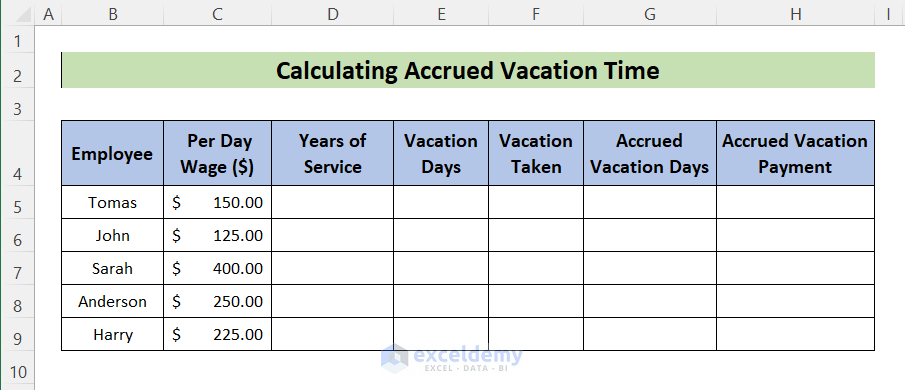
Step 1: Create Paid Time Off (PTO) Structure
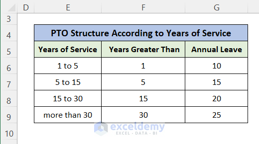
At first, you have to make a PTO structure for your company as per the years of service given by the employee. As the senior employees will get more leave days than the new joiners.
- So, create a table containing the permitted paid leave days for employees concerning their years of service.
- Create one more column that contains the lower of the group range for the years of service. This column will be used for the VLOOKUP formula.
Read More: How to Create Leave Tracker in Excel (Download Free Template)
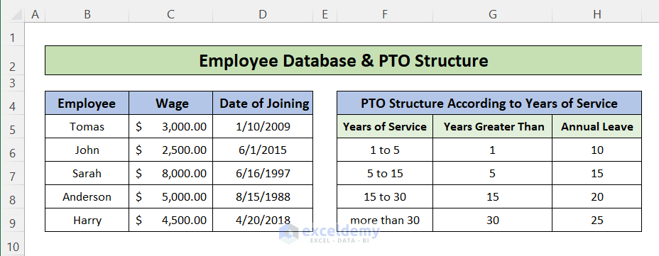
Step 2: Create Employee Database with Joining Dates
Then, you should have a ready database of employee data. Collect the data of employee names, joining dates, and wages. And, make a table with these data in an Excel worksheet.
Read More: Employee Leave Record Format in Excel (Create with Detailed Steps)
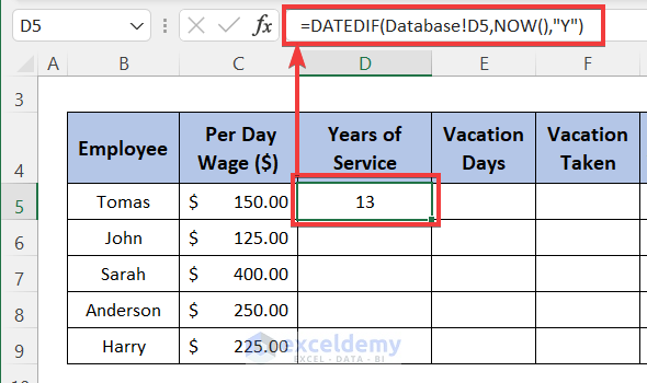
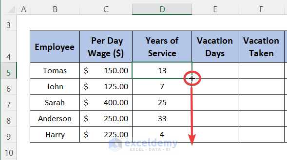
Step 3: Calculate Years of Service
Now, you have to calculate the years of service given by the employee. You can use the DATEDIF function to calculate the years from the joining date till today. For this, paste this link into cell D5:
=DATEDIF(Database!D5,NOW(),"Y")
Formula Explanation
- Start_date = Database!D5
This will give the joining date of the respective employee from the Database sheet. - End_date = NOW()
To get the date of the working date, the NOW Function is used here. - Unit = "Y"
It will give years between the two dates.
- Now drag the Fill Handle icon to paste the used formula respectively to the other cells of the column or use Excel keyboard shortcuts Ctrl+C and Ctrl+P to copy and paste.
Read More: How to Calculate Annual Leave in Excel (with Detailed Steps)
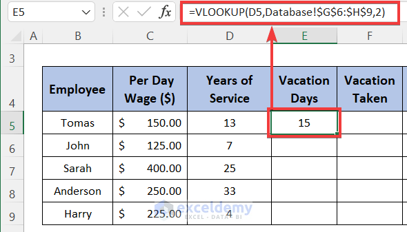
Step 4: Calculate Allowed Vacation Days
Now, to get the allowed leave days of employees concerning their joining date of them, you have to use the VLOOKUP function in Excel. So, paste this link into the cell E5:
=VLOOKUP(D5,Database!$G$6:$H$9,2)
Formula Explanation
- Lookup_value = D5
The function will look for the value in cell D5 in the lookup table - Table_array = Database!$G$6:$H$9
This is the range of cells which is the lookup table where the function will search for the lookup value. - Col_index_num = 2
It will return the value of column 2 in the lookup table from the row where the lookup value exists.
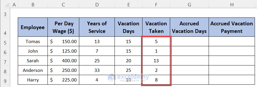
Step 5: Insert the Number of Vacation Days Taken from Employees' Attendance Tracker
Now, open the Employee attendance tracker of that year and link the cell containing the total leave days taken with this file in cell F5 or insert the values manually in the vacation taken column.
Read More: Employee Monthly Leave Record Format in Excel (with Free Template)
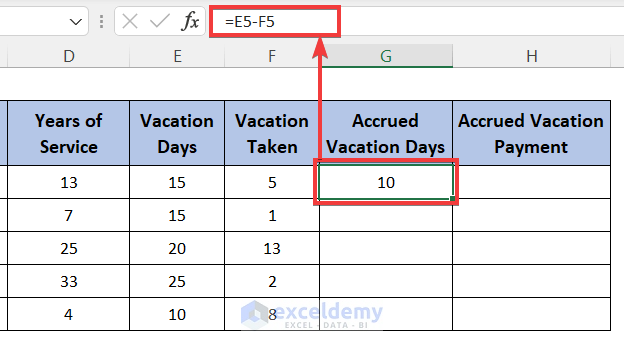
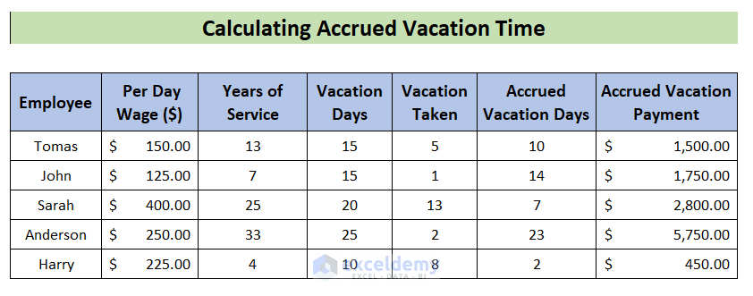
Final Step: Calculate Accrued Vacation Time
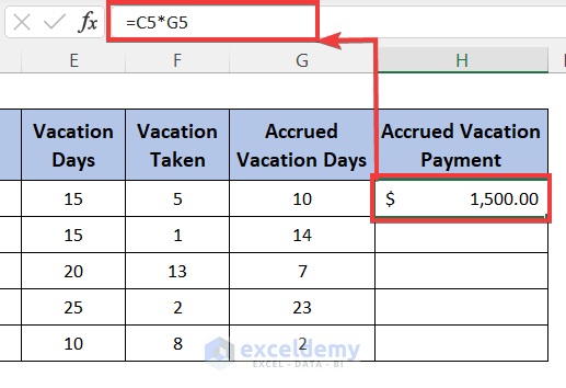
Now, calculate the accrued vacation days with this formula:
Accrued Vacation Days = Allowed Vacation Days – Vacation Taken
Now, you can calculate the accrual vacation payment to encash the leave days not taken. So, the formula will be:
Accrued Vacation Payment = Accrued Vacation Days x Daily Wages
Now, you have the accrued vacation days and the payments of the employees of your company.
Calculate Accrued Vacation Time in Excel Excluding Probationary Period
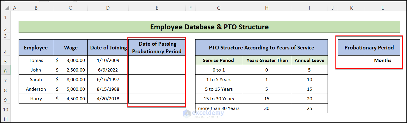
In most companies, the accrued vacation time is calculated excluding the probationary periods. During the probationary period, there is no paid leave facilities. So, during the calculation of accrued vacation, we have to take the passing date of the probationary period as the starting date of service. Here, I am showing you the steps on how you can calculate the accrued vacation time for companies that follow the probationary period policy.
📌 Steps:
- First, insert a new column to calculate the date of the passing period of the probationary period. And, assign a cell to get input of the months of the probationary period.
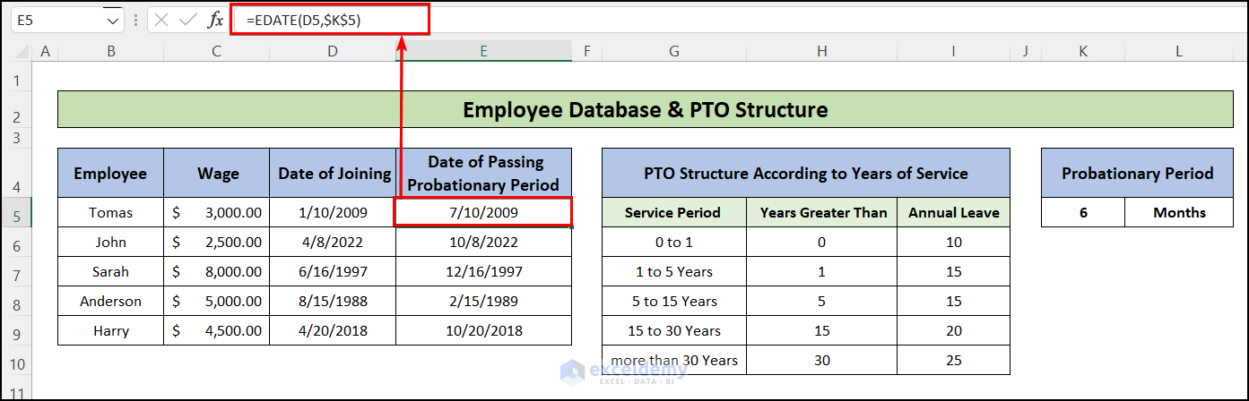
- Then, insert the following formula into cell E5 and drag the fill handle till the last row of the table
The EDATE function gives the date value after adding a given number of months. Here, It is adding 6 months which is the probationary period with the joining date, and gives the passing date.
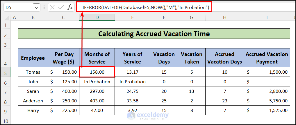
- Then, go to the "Accrued Vacation" worksheet and rename column D as "Months of Service". Also, add a new column after that named "Years of Service".
- Then, insert the following formula into the cell D5:
=IFERROR(DATEDIF(Database!E5,NOW(),"M"),"In Probation")
The IFERROR function returns "In Probation" if the end date in the DATEDIF functionis after the present date. And, for these rows, you don't have to calculate the accrued vacation time.
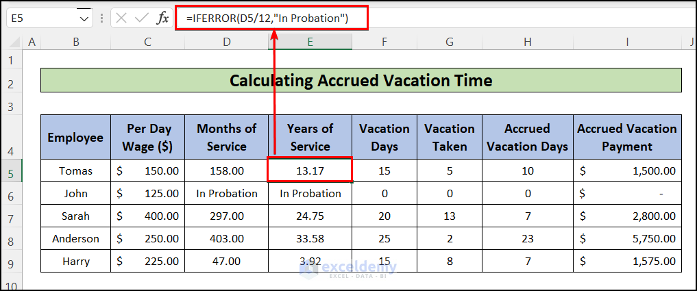
- Now, calculate the years of service using the following formula in cell E5, and, drag the fill handle to apply similar formula for other cells also.
=IFERROR(D5/12,"In Probation")
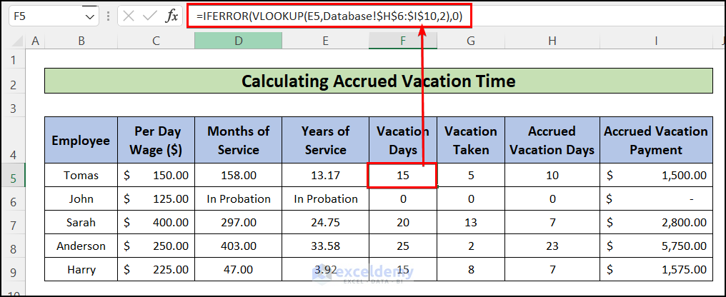
- After that, insert the following formula to get the allowed accrued vacation time for the employees in cell F5:
=IFERROR(VLOOKUP(E5,Database!$H$6:$I$10,2),0)
- Calculate the remaining part using the similar steps mentioned in the Final Step of the previous method.
Conclusion
In this article, you have found how to calculate accrued vacation time in Excel. Download the free workbook and use it to make an annual vacation accrual spreadsheet template for your company. I hope you found this article helpful. You can visit our website ExcelDemy to learn more Excel-related content. Please, drop comments, suggestions, or queries if you have any in the comment section below.
Related Articles
- How to Calculate Leave Balance in Excel (with Detailed Steps)
- How to Calculate Half Day Leave in Excel (2 Effective Methods)
Source: https://www.exceldemy.com/calculate-accrued-vacation-time-in-excel/
0 Response to "Starting Paid Time Off at 80 Hours and Continual Accrual of 466 Biweekly"
Post a Comment